These readings are recommended for my Electroaccoustic Engineering Course students.
A CLEAN AUDIO INSTALLATION GUIDE™

BENCHMARK’S «CLEAN AUDIO INSTALLATION GUIDE™«
By Allen H. Burdick
«REQUIRED READING!»
 This 24 page guide has been very popular. It has been hailed as “required reading for all broadcast engineers” by Richard Sequerra.
“We were able to change our engineering standards throughout the CBC as a result of this paper.” – Tom Holden Manager, Systems Engineering – Radio, CBC Toronto.
This paper revolutionized broadcast audio in the 1980’s. It moved the industry away from 600-Ohm interfaces and radically changed the way analog audio was handled in professional environments.
In many ways, this paper still impacts every product that Benchmark builds today. We think that you will find this classic paper as useful today as it was when it was originally published in the 1980’s. Due to the popularity of this paper, Allen updated it several times. The links will take you to Allen’s final 1997 version.
We agree with Richard Sequerra. This is your required reading assignment!
RULES OF THUMB FOR MUSIC AND AUDIO

by John Siau
As an engineer I like to use «rules of thumb» to make quick estimates that help explain what can be expected from the physical world around me. These rules of thumb are easy-to-remember approximations that eliminate the need for complicated and needlessly precise calculations.
If you learn a few key rules of thumb, you can gain a tremendous understanding of the world around you. For those of you who feel discombobulated by the complexities of high school physics, there is hope! I encourage you to step back and take a fresh look at the world around you. If you learn a few simple rules of thumb, you can begin to unravel the mysteries of physics while amazing your friends and yourself.
In this paper I will present 15 simple rules that I find useful when working with audio. I have assigned numbers to each in order to make the discussion clearer. Memorize the rules, not the rule numbers.
Let’s begin with a simple but very fundamental rule of thumb: We all know that light travels at some ridiculously fast speed, but we seem to have a hard time expressing this speed in terms of meaningful numbers. How many of you physics gurus can even remember the speed of light in MPH, ft/sec, or m/sec? OK, try this:
Rule 1: Light and electrical signals travel about 1 foot in 1 ns.
1 ns (nanosecond) is 1 billionth of a second. The exact speed of light is closer to 1.018 feet in 1 ns in a vacuum, and it is nearly the same in air. As rules of thumb go, this one is unusually precise! Electrical signals flow through a wire at a slightly slower rate, (0.5 to 0.95 times light speed), but this rule of thumb is accurate enough to include most estimates relating to electrical signals.
Let’s compare the speed of light to the speed of sound:
Rule 2: Sound travels about 1 foot in 1 ms.
1 ms (millisecond) is 1 thousandth of a second. The exact number is is closer to 1.125 feet in 1 ms. This rule of thumb has more than a 12% error, but it is useful because it is easy to remember and it is accurate enough for most quick estimates. Rules of thumb do not need to be precise, they just need to be easy to use. In most quick estimates, this 12% error is not important.
The main lesson from these first two rules of thumb is that light travels about 1 million times faster than sound! This gives us our third rule of thumb:
Rule 3: Light travels 1 million times faster than sound.
Rule 3 tells me that electricity travels to my speakers about a million times faster than the sound they produce. This tells me that it is far more important to match the distance to my left and right speakers than to match the lengths of my speaker cables.
RULES 2 AND 3 CAN SAVE YOUR LIFE!
 Rule 3 tells me that if I see a lightning strike in the distance, the time is takes for the light to arrive is insignificant. It is only 1 millionth of the time it takes for the sound to arrive. This means that I can ignore the time it takes for the light to arrive. I can estimate the distance by measuring the time it takes for the sound to arrive. I simply measure the time between seeing the flash and hearing the boom. Rule 2 gives me the answer: Every second is about 1000 feet. Five seconds is about a mile.
Notice that I am taking the liberty of rounding a mile to 5000 feet. When making quick estimates, using rules of thumb, feel free to round the numbers and make the math easier. Remember, we use rules of thumb to make quick estimates. Keep the math as simple as possible!
For the lightning strike estimate, my rules of thumb are probably much more accurate than my ability to count the seconds from the strike. For this reason, using the exact 1,125 ft/s number is not really necessary. Exact numbers are harder to remember and they complicate the calculations. Keep it simple, and you will gain more understanding of the world around you! The laws of physics can be simplified so that they can become a meaningful part of your daily life. When lightning is striking nearby, a quick estimate is much more useful than a precise calculation!
HOW DO RULES OF THUMB RELATE TO MUSIC AND AUDIO?
 If we look at musical instruments, we can learn many things by applying Rule 2 (the speed of sound). Nothing is more central to the physics of music than the speed of sound. For example, we can create musical instruments from resonant tubes and chambers that derive their pitch from the time it takes for sound to traverse the chamber or tube. The resonant space could be a soda bottle, flute, trumpet or organ pipe. Any confined space will resonate at specific frequencies that are determined by the size of the chamber and by the speed of sound.
 Stringed instruments often have chambers that are intended to add resonance at a wide variety of frequencies. These chambers have complex shapes so that they will have resonant modes at many different frequencies. When stimulated by a source of noise, resonant frequencies are amplified by the chamber.
Our listening rooms also form resonant chambers, and our rules of thumb will help us to understand the resonant characteristics of our room. We can do this by considering three separate 2-dimensional reflection paths: Front to back wall, side to side, and floor to ceiling. Lets begin by constructing a 2-dimensional resonator with a piece of pipe. After we understand this 2-dimensional resonator, we can estimate the resonance of 3-dimensional spaces.
MAKING MUSIC WITH PIPES
 If we construct a pipe that is closed at both ends, it will resonate at a frequency that is determined by the time it takes sound to go down to the far end and reflect back to the near end. In other words, a tube with closed ends will resonate when sound travels down and back in exactly one cycle of the stimulus tone. If both ends are open, the reflections still occur and tube still resonates at the same frequency.
If we build a 2-foot long organ pipe with open ends , Rule 2 tells us that it will take about 2 ms for the sound to travel down the tube and 2 ms for it to make the return trip. In the span of one second, sound can make this round trip about 250 times. This means that the tube will resonate at about 250 Hz (250 cycles per second, or 250 down and back trips per second). If we do a more precise calculation (using 1,125 ft/s) we arrive at our next rule of thumb:
Rule 4: A 2-foot open pipe resonates at 262 Hz which is middle C.
Just remember «2, 262, middle C».
If you prefer, you can round the frequency to 250 Hz whenever you want to make the math easy. 250 Hz is about midway between B and C on the piano, so you can make quick approximations and still estimate which note will be played.
RULE 4 IS AN OLD RULE OF THUMB

An organist or an organ builder would be very familiar with Rule 4. Most could instantly tell you that a two-foot pipe produces middle C. Pipe organ stops enable groups of pipes, which are called ranks. The stop for each rank is labeled according the approximate length of the longest pipe in the rank. Note the numbers 2, 4, 8, or 16 under the name of the various stops in the photo to the left. This German pipe organ dates from the Baroque period (17th to 18th century).
Most ranks begin with a C pipe. The lowest pipe in a «2-foot» rank plays middle C (262 Hz). A 4-foot rank begins one octave below middle C (131 Hz), an 8-foot rank begins two octaves below middle C (65.4 Hz), and a 16-foot rank begins 3 octaves below middle C (32.7 Hz). Some pipe organs include 32-foot ranks which begin 4 octaves below middle C (16.35 Hz).
There are two pipe organs in the world that include 64-foot ranks. These play a very low C at about 8.2 Hz. You must experience these organs in person to hear and feel these lower notes. In many cases, we hear the harmonics of the resonant frequency while feeling the vibrations of the fundamental. It would be difficult to build an audio system that could reproduce the experience produced by 32 and 64 foot ranks! It would also be hard to fit such a system into your living room.

Organ Console in Cadet Chapel at West Point Military Academy – Largest chapel pipe organ in the world, 23,511 pipes – photo by John Siau
WHAT ARE HARMONICS?
Harmonics are integer multiples of the fundamental tone. If 10 Hz is the fundamental resonant frequency, the harmonics are 20 Hz, 30 Hz, 40 Hz, and so on. These are called the 2nd, 3rd, and 4th harmonics respectively. In our example 262 Hz (C4) is the fundamental, 524 Hz (C5) is the 2nd harmonic, and 786 Hz (G5) is the third harmonic. Pipes will resonate at harmonics of the fundamental when stimulated with harmonics.
DON’T CONFUSE HARMONICS WITH OCTAVES.
The 2nd harmonic is one octave above the fundamental, but the 3rd harmonic is not the next octave step. The 2nd harmonic is an octave step because it is twice the frequency of the fundamental. The next doubling in frequency gives us the 4th harmonic which is two octaves above the fundamental. Another doubling in frequency will give us the 8th harmonic which is three octaves above the fundamental. If you are following the pattern here, you can see that the next octave would be the 16th harmonic. The sequence is 1, 2, 4, 8, 16, … This group of even harmonics are perfect octaves and this makes them very musical. The remaining even harmonics (6, 10, 12, 14, 18, …) also tend to be more musical than the odd harmonics.
Nevertheless, odd harmonics play an important part in giving musical instruments their timbre. Unique blends of odd and even harmonics give different instruments their distinct timbre. The construction of organ pipes can be varied to achieve a wide variety of sounds. A large pipe organ will have a vast selection of different sounds produced by ranks of pipes having different styles of construction. The differences in timbre can be attributed to the difference in the harmonic content produced by various types of pipes.
Most musical instruments produce significant harmonic content when a note is played. To preserve the unique timbre, audio systems must accurately reproduce these distinct harmonic patterns without adding harmonic distortion.
EXPONENTIAL CHANGES IN SIZE
 The main takeaway here is that the size of musical instruments change very rapidly over the range of a few octaves. Compare the size of a tuba to the size of a trumpet which plays just two octaves higher. Compare the size of a flute to the size of a piccolo. A flute is roughly 26″ long and a piccolo is roughly 13″ long. This 2:1 reduction in size makes a piccolo play exactly one octave higher than a flute.
Every time the pipe length is cut in half, we increase the pitch by one octave. If we want to decrease the pitch by an octave, we will need to increase the length by a factor of two. This brings us to our next rule:
Rule 5: An octave change in pitch requires a 2:1 change in size. Bigger is lower.
Every doubling in length cuts the resonant frequency (pitch) in half. Think about our two foot long organ pipe. If we make this twice as long, the sound will need to travel twice a far for each round trip. The sound can only make half as many round trips in a given time period. In our two-foot pipe, the sound could make 262 round trips per second. In a four-foot pipe, sound can only make 131 round trips per second. 131 Hz is C3 on the piano. It is one octave lower than middle C. If we make the pipe 4 times as long, the frequency will drop by a factor of 4 which is two octaves lower.
Nobody really needed to tell you this! You learned this when you carried groceries into the house for your mom. If she parked the car twice as far away, it would take you twice as long to make each trip. You would arrive at the door less frequently. The frequency of your round trips was determined by the distance you had to travel.
Rule 6: A piano has a range that exceeds 7 octaves.
 The fundamental frequencies of an 88-key piano range from a high of 4186 Hz (C8) to a low of 27.5 Hz (A0). This is a 152:1 ratio in frequency which implies a 152:1 ratio in size. This explains the size variations in musical instruments and it explains the size differences between woofers and tweeters in an audio system.
If we wish to build an organ that just matches the range of the piano, the shortest pipe would be an inch and a half long while the longest pipe would be over 8 feet long. As stated above, large pipe organs extend the low range beyond that of the piano by adding 16-foot, 32-foot or even 64-foot pipes. Pipes for high notes can be overblown so that they resonate an octave or two higher than the fundamental and this allows the use of longer pipes for some of the higher notes.
Pipe organs represent a fascinating blend between music, and engineering. Some of this engineering dates back to the 3rd century BC. Between the 17th and late 19th centuries, no man-made device was more complex than the pipe organ.
Our Rule 4 and Rule 5 were well known to the builders of these early pipe organs. We can use these same rules of thumb to analyze 3-dimensional spaces.
ESTIMATING ROOM RESONANT FREQUENCIES
We can use Rule 4 and Rule 5 to estimate resonant frequencies within our listening room. Sound bounces between parallel surfaces in our room just like it bounces off of the two ends of a pipe. We have a resonator formed between the front and back walls. We have a second resonator formed between the two side walls. A third, and often forgotten resonator, is formed between the floor and the ceiling. If we are unlucky enough to have a listening room that is shaped like a cube, all three resonators will be tuned to the same fundamental frequency (and its harmonics).
Let’s suppose we are unlucky and our listening room is a 10 foot cube. From Rule 4 we know that a 2 foot distance would give us a resonance at 262 Hz. We will round this to 250 Hz, just to keep the math simple.
Since 10 feet is 5 times as far as 2 feet, the resonant frequency will drop by a factor of 5 (five times as far, one fifth as many round trips per second). The resonant frequency will be approximately 250 Hz/5 = 50 Hz. 50 Hz is approximately the 9th key from the bottom of the piano keyboard. The room would also resonate at the harmonics of 50 Hz (100 Hz, 150 Hz, 200 Hz, 250 Hz …). If you were to place a piano in your 10-foot cube, you could expect that the notes corresponding to these frequencies would sound much louder than many of the other notes on the piano. It could be difficult to enjoy listening to a piano in this cubic room.
We could try to mitigate these resonant frequencies by adding lots of absorptive material to the walls, floor, and ceiling, but this could be expensive. It also takes very thick material to absorb low frequencies. In practice, we would only be able to absorb some of the higher harmonics. It would be extremely difficult to absorb the 50 Hz fundamental resonance.
 If we were building a space for listening to music, we would want to avoid building a cube. Ideally we should select dimensions that interleave the resonant frequencies. We should also avoid integer ratios between the dimensions.
We may also want to avoid creating large parallel surfaces. Most recording studios have walls and ceilings that are angled relative to each other. Studios also avoid large flat surfaces. If possible, eliminate parallel surfaces, and break up large flat surfaces. Random and irregular surfaces diffuse the reflections that would otherwise cause resonant frequencies. Absorptive materials can reduce the severity of the resonant frequencies, especially at high frequencies.
Given Rules 4 and 5, you can estimate resonant frequencies in your listening room. These simple rules will help you to determine problem frequencies in your room. If you want precise answers, there are a number of room-modes calculators on the internet that can be used to do a complete analysis of the resonant modes of a room. Many of these tools can suggest a set of dimensions. Use these tools before you build your new listening room!
RULES-OF-THUMB RELATING TO LOUDNESS
As we think more about audio, it is clear that we must have some understanding of decibel units and why we use them. It turns out that our ears have an amazing dynamic range. We can hear a mosquito on the other side of the room and we can tolerate sound of a clap of thunder. There is a 1 trillion to one power ratio between these two sounds! There is actually a 10 trillion to one power ratio between the loudest sounds we can tolerate and softest sounds we can hear.
Our ears have a logarithmic response to audio power. Fortunately, a clap of thunder doesn’t sound a trillion times louder than a mosquito. The logarithmic response or our ears provides us with a tremendous ability to extract details from loud and soft sounds. We could express loudness on a linear scale ranging from 1 to 10 trillion, but this would be cumbersome and hard to decipher. For this reason, logarithmic units are usually the best choice for audio loudness measurements, calculations, and specifications. 130 dB is an easy way to express the 10,000,000,000:1 power ratio that corresponds to the dynamic range of the human ear. As we explore the concept of decibels (dB), we will discover some very useful rules of thumb:
Rule 7: 0 dB SPL is the threshold of normal hearing.
A sound at 0 dB SPL is just loud enough to be heard. It is roughly equivalent to the sound of a mosquito flying 10 feet (3 m) away. This threshold of hearing is frequency dependent and listener dependent. Most listeners with normal hearing have maximum sensitivity at about 3 kHz. This sensitivity tapers off above and below 3 kHz. Use the 0 dB SPL threshold for quick approximations of audibility especially when considering mid-range sounds.
SPL is an abbreviation for sound pressure level. It is measured in dB relative to a reference pressure level that corresponds to the threshold of hearing.
Rule 8: 130 dB SPL is about the highest peak loudness that we can tolerate.
Very brief exposures at this level can cause permanent hearing damage. OSHA allows less than 2 minutes of exposure per work day at 130 dB SPL. The threshold of pain may be as high as 140 dB for some listeners but this threshold also varies with frequency. Curiously, the threshold of pain tends to get lower after our ears have sustained permanent damage. Some listeners may experience pain at much lower levels.
In the context of a home audio system, there is no sane reason for having the ability to produce peak sound pressure levels above 130 dB SPL at the listening position. If your sound system is hitting your ears with 130 dB SPL on very short peaks it is almost certainly playing at ear-damaging levels.
 In a very large room or an outside venue, a sound system may need to produce sounds above 130 dB SPL (at the speakers) in order to achieve reasonable levels at the listening position.
Rule 9: A 1 dB change in loudness is a just noticeable difference (JND).
At mid loudness levels, a 1-dB change in loudness is just noticeable. A 1-dB increase requires a 25% increase in power. At higher loudnesses, changes as small as 1/3 dB may be noticeable. The JND threshold also varies with frequency. Nevertheless 1 dB is a good rule of thumb.
Benchmark products have volume controls with 1/2 dB steps. This allows an adjustment in level that is just noticeable. Smaller steps would serve no useful purpose.
Rule 10: A 3 dB increase in loudness requires a 2X increase in power.
A 200 W power amplifier is just 3 dB louder than a 100 W amplifier.
Rule 11: A 6 dB increase in loudness requires a 4X increase in power which is a 2X increase in voltage.
 A stereo amplifier running in bridged mono mode will produce twice the voltage and can produce up to four times the power into a given load. The Benchmark AHB2 power amplifier is about 6 dB louder when running in bridged mono mode.
Rule 12: A 10 dB increase in loudness requires a 10X increase in power.
From this we can see that a 100 W amplifier will play 10 dB louder than a 10 W amplifier.
Rule 13: In a home environment, the SPL at the listening position is about the same as the 1m response of the speaker in an anechoic chamber.
If a speaker has a measured output of 90 dB SPL at 1 meter when fed with one watt, you can expect about 90 dB SPL at your listening position when driving your speaker with one watt. Room reflections supplement the output of the speakers and compensate for the fact that you are more than 1 meter from your speakers. If you are outdoors, this rule does not apply. But, in a typical home listening room, the rule works reasonably well for a quick approximation.
Rule 14: Every bit in a digital system adds 6 dB to the signal to noise ratio (SNR) of the digital channel.
The actual formula is (6.02 dB * n) + 1.76 dB where n is the number of bits. Subtract 4.77 dB if TPDF dither is used. This means that a 16-bit system provides a SNR of between 93.31 and 98.08 dB depending upon the use of dither. Our rule of thumb gives us 96 dB which is right in the middle of this range. In all cases, adding 1 bit increases the SNR of the digital channel by exactly 6.02 dB when it is measured over the entire bandwidth of the digital channel. Don’t get bogged down in the details, the 6 dB per bit approximation is a very good rule of thumb.
Rule 15: The bandwidth of a digital system is 1/2 of the sample rate.
The 44.1 kHz sample rate used on CDs provides a 0 Hz to 22.05 kHz frequency range. Frequencies above 22.05 kHz cannot be recorded on a CD. One half of the sample rate is also known as the Nyquist frequency. Frequencies below the Nyquist frequency can be digitized and reproduced accurately.
USE YOUR RULES OF THUMB TO CHECK HIGH-PRECISION CALCULATIONS!

It is easy to make mistakes when making precise calculations. Check your work against quick estimates based upon rules-of-thumb that you have memorized or learned through experience. Is the calculated result about what you expected? If your precise calculations differ from your quick estimates by more than a reasonable margin, it is time to go back and check the math.
If you want to travel from Boston to New York, you may know from experience that this should take about 4 hours. From prior experience, you have developed a rule of thumb for trips between these two cities. If you plug this trip into Google maps and get 72 hours, you know something is wrong! It could be that Google thinks you are walking. Click on the car icon and try again.
– John SIau
BALANCED VS. UNBALANCED ANALOG INTERFACES


If you look at the back of any Benchmark product, you will find balanced XLR analog-audio connectors. As a convenience, we also provide unbalanced RCA connectors on many of our products. In all cases, the balanced interfaces will provide better performance.
We build our unbalanced interfaces to the same high standards as our balanced interfaces, but the laws of physics dictate that the balanced interfaces will provide better noise performance.
This paper explains the advantages of balanced interfaces as compared to unbalanced.
NOISE SOURCES
There are several sources of noise that can contaminate the audio when two audio products are connected together with a cable. These noise sources include ground loops, radio interference, magnetic interference, thermal noise and noise from the input and output buffers.
SIGNAL TO NOISE RATIO (SNR)
The signal to noise ratio (SNR) is the ratio between the maximum signal voltage and the idle-channel noise voltage. This ratio is usually expressed in dB. The higher the ratio, the better the performance. To keep noise completely inaudible, the A-weighted SNR in dB should exceed the peak sound pressure level (SPL), at the listening position, expressed in dB SPL. When this condition is satisfied, the noise will be below the 0 dB SPL threshold of normal hearing.
The peak sound pressure should not be confused with the average levels read by an SPL meter. The peak level will be substantially higher but can be calculated from the amplifier output voltage and the speaker efficiency. This calculation is covered in some of my other application notes.
Most audio systems produce some audible noise. In other words the noise level emitted from the loudspeakers exceeds 0 dB SPL. Many listeners have accepted this distraction as a necessary part of audio electronics, but the technology exists to produce entire systems that emit no audible noise. Balanced interfaces are one important feature of these state-of-the-art systems.
SNR OF AUDIO INTERFACES
In this paper we will be focusing on the capabilities of the interfaces that connect audio components together to form a system. In many systems, the interfaces limit the noise performance of the overall system. To avoid this limitation, the interfaces should provide better performance than the poorest performing component in the signal chain.
NOISE FIGURE
If we want an interface to impose no more than a 1 dB reduction on the system SNR, it will need to have an SNR that is at least 6 dB better than the lowest performing device in the signal chain. If a noise source causes a 1 dB reduction in noise performance, we call this a 1 dB «noise figure».
If our interface SNR is 12 dB better than the worst component in our system, then the interface will impose a 0.27 dB noise figure on the system. 12 dB is a 4:1 ratio. At this 4:1 ratio of component noise to interface noise, the interface still causes a slight reduction in the system SNR. This demonstrates the need for interfaces that are much quieter than the devices they connect.
EXAMPLE – CONNECTING A DAC TO A POWER AMPLIFIER
If we connect a Benchmark DAC3 (128 dB A-weighted SNR) directly to a Benchmark AHB2 monoblock amplifier (135 dB A-weighted SNR) we should be able to achieve a system SNR of about 127 dB. The SNR of the AHB2 is 7 dB better than that of the DAC3 so it will impose a noise figure of just less than one dB on the DAC3.
To avoid more than an additional dB increase in noise, the interface between the two boxes will need an SNR that is at least 6 dB better than the combined 127 dB SNR. This means that the interface needs to have an SNR of at least 133 dB. If we attempt to use the 2 volt (8.2 dBu) RCA output on the DAC3, we will not achieve the desired result. If you do the math (8.2 dBu – 133 dB) , the unbalanced outputs and inputs would need to achieve a noise level of -124.8 dBu. This is nearly impossible because this is equivalent to the thermal noise produced by a 600-Ohm resistor. The unbalanced input and output stages would need to use very low impedances and we would need to hope that we didn’t pick up any additional noise from ground-loop interference.
In our example, the upstream unbalanced output on the DAC3 would be the limiting factor in terms of noise. The DAC3 has high-quality low-noise unbalanced outputs, but these cannot support the full 128 dB SNR of the DAC3. Under ideal lab conditions, we would suffer about a 10 dB reduction in system SNR when connecting the DAC3 to the AHB2 using the unbalanced outputs on the DAC3. Outside of the lab, ground-loops and electromagnetic interference (EMI) could add additional noise to this unbalanced interface.
If we use the balanced outputs on the DAC3, this interfacing task is easy and we will achieve our system SNR goals while adding immunity to interference.
WHY ARE THERE NO UNBALANCED INPUTS ON THE AHB2 POWER AMPLIFIER?
If you look at the back of the AHB2 you will see that there are no unbalanced inputs. Unbalanced inputs have no business being on a device that delivers a 135 dB SNR. Unbalanced interfaces operate at 2 Vrms which is about 8.2 dBu. If you do the math (8.2 dBu – 135 dB – 6 dB), you will find that the noise on the interface would need to be -132.8 dBu to achieve a 1 dB noise figure. To put this in perspective, a single 91-Ohm resistor produces a thermal noise level of -132.8 dBu, and the best microphone preamplifiers have an equivalent input noise (EIN) of about -130 dB. If we want to use 2 Vrms input levels, we would need an input amplifier that is better than any microphone preamplifier ever built! Due to the laws of physics, this requirement is impossible to achieve.
The only solution is to use higher signal levels. These are only available from balanced outputs.
For compatibility with consumer equipment, the AHB2 has three input gain settings: The high-gain mode supports 2 Vrms inputs, the mid-gain mode supports 4 Vrms inputs, and the low-gain mode supports professional +24 dBu (12.28 Vrms) inputs. To achieve maximum performance, it is essential to feed the amplifier with professional studio-level inputs while using the low-gain setting.
INCREASE THE SIGNAL LEVELS
One of the easiest ways to improve the SNR of an interface is to increase the signal level. For example, if we double the signal voltage, we are increasing the level by 6 dB and this increases the SNR of the interface by 6 dB.
STUDIO-GRADE BALANCED INTERFACES
Professional balanced interfaces generally operate with much higher signal levels than unbalanced consumer interfaces. This voltage difference gives these balanced interfaces a significant SNR advantage over unbalanced interfaces. Most RCA interfaces operate at a maximum signal level of +8.2 dBu which is 2 Vrms. In contrast, professional balanced interfaces usually operate at a maximum signal level of +24 dBu which is 12.28 Vrms. If you do the math (24 dBu – 8.2 dBu) you can see that the signal level is 15.8 dB higher on the professional-grade balanced interface. If the noise is the same on both interfaces, the balanced interface will provide almost a 16 dB improvement in the interface SNR.
But, balanced interfaces always require dual output buffers and dual input receivers. These additional active devices contribute some noise and this tends to reduce the SNR improvement by about 3 dB. Taking this into consideration, the interface SNR of a professional balanced interface is still about 13 dB better than that of an unbalanced consumer interface.
In addition, balanced interfaces provide rejection of many types of interference. This immunity to interference can provide a 50 to 100 dB reduction in these unwanted noises. This immunity to interference is usually more than enough to keep the interference inaudible.
Professional interfaces are more expensive to build. The high signal levels generally require the use of +/- 18 volt power supplies within the audio product. To save costs and reduce the power consumption, consumer products usually use much lower supply voltages. As a result, it is rare to find consumer audio products with balanced interfaces that can support professional signal levels. These products have dumbed-down balanced interfaces that operate at much lower voltages.
CONSUMER-GRADE BALANCED INTERFACES
Many high-end consumer products have balanced interfaces, but they operate at a maximum level of 4 Vrms which is + 14.2 dBu. This is 10 dB lower than the level used in professional interfaces. This means that the 13 dB advantage provided by a +24 dBu balanced interface is reduced to just 3 dB when operating at a maximum level of +14.2 dBu. Consumer-grade balanced interfaces are definitely a step better than unbalanced interfaces, but the signal levels are too low for use in very high perfomance systems.
Benchmark D/A converters are equipped with professional-grade +24 dBu outputs. These outputs have 10 dB passive pads that can be engaged in order to drive consumer-grade 4 V balanced inputs. If you find you need these pads, it is a good indication that the downstream device is limiting the SNR performance of your system. Likewise, the AHB2 has a gain setting that supports inputs from 4 Vrms consumer-grade balanced outputs. Again, these consumer-grade devices will be the weak link in the system.
Check the specifications and look for balanced interfaces that support professional signal levels. Consumer-grade balanced interfaces may look like professional interfaces, but they do not provide the same level of performance.
COMMON-MODE NOISE REJECTION
The largest benefit of balanced interfaces comes from their ability to reject common-mode noise signals. Balanced input receivers have active differential amplifiers or passive transformers that respond to the difference between the + and – input pins. The ground pin on the XLR connector is only used for shielding. The ground connection is not part of the audio signal and it is ignored by the input amplifier or input transformer.
Ground currents, and differences in ground voltage, can create noise signals that are identical on both the + and – pins. This common-mode noise will cancel and be rejected by a transformer or a well-trimmed differential amplifier.
CMRR
The common-mode rejection ratio (CMRR) is a measure of how well a balanced receiver rejects common-mode noise. A high CMRR is an indication that the balanced receiver will reject most of the noise voltage caused by ground loops and other sources of common-mode interference. Transformers generally provide very a high CMRR but may add distortion and frequency response problems. Active differential amplifiers can provide better transparency than transformers and can provide a very high CMRR if they are well trimmed.
Good differential amplifiers provide at least 50 dB of rejection at AC line-related frequencies. This is usually enough to reduce AC ground loop interference to inaudible levels. Well-trimmed differential amplifiers, such as those used in Benchmark products, may provide a CMRR of 70 to 100 dB at AC line-related frequencies.
DIFFERENTIAL AMPLIFIERS – THE KEY COMPONENTS IN BALANCED RECEIVERS
There are some consumer products that have «balanced» inputs with a CMRR of 0 dB. Let’s just call these «fake» balanced inputs. The input is equipped with an XLR connector, but the – pin (pin 3) is ignored. These are just unbalanced inputs wired to an XLR connector. They offer no advantage over unbalanced RCA inputs. In most cases, pin 2 of the XLR is tied directly to the center contact of a nearby RCA input. This makes the XLR jack nothing more than an adapter.
There are other devices that use the + and the – pins, but they fail to remove common mode noise before the signal leaves through a balanced output. These devices simply pass the common mode noise on to the next component in hopes that the next component will remove the common mode noise. If you can’t find a specification for CMRR, the balanced input may not have a differential amplifier. If this is the case, the input is just a pair of unbalanced inputs feeding a pair of unbalanced outputs.
DIFFERENTIAL AMPLIFIERS IN D/A CONVERTERS
High-quality D/A converter chips use balanced outputs. The purpose of these balanced outputs is to increase the signal level by a factor of two (6 dB) while providing a means for removing the common-mode distortion produced by the converter chip. This common-mode error tends to be odd-harmonic distortion and is not musically pleasing. This low-level distortion can change the character of musical voices and detract from the music. This common-mode distortion is only removed if the D/A converter feeds a well-trimmed differential amplifier.
I have seen many D/A converters that completely omit the differential amplifier. This omission is actually common practice in most «high-end» D/A converters. Unfortunately this leads to very unpredictable performance. The D/A converter will still measure well when it is connected to the balanced input on an audio analyzer, but may not perform nearly as well in a typical system. A good analyzer will always have an excellent CMRR and this will reject the common-mode distortion produced by the D/A converter chip. In a real system, the D/A converter could be driving a balanced input with a poor CMRR and the common-mode distortion would not be rejected. Furthermore, If this D/A converter also has unbalanced outputs, these outputs will be contaminated with distortion that could have been removed by a differential amplifier. Once this distortion reaches an unbalanced output, it cannot be removed by a downstream device.
To avoid these problems, Benchmark D/A converters include well-trimmed differential amplifiers to remove the converter common-mode distortion before it reaches any of the outputs. From a distortion standpoint, the balanced and unbalanced outputs on a Benchmark D/A converter will have identical THD performance. But, from a noise standpoint, the balanced outputs provide better performance.
SOLVING GROUND LOOP PROBLEMS
In a balanced system, ground loops generate common-mode noise, and balanced receivers can provide near-perfect (50 dB to 100 dB) rejection of this troublesome noise. For this reason, balanced interfaces are considered absolutely essential in professional environments.
Balanced interfaces are also the solution to the many ground loop problems that occur in a complex home hi-fi system. Cable boxes, TV antennas, computer USB ports and AC ground pins may all be at different ground potentials. By code, cable TV and antenna cables must be grounded where they enter the building. These ground points are rarely the same as the ground delivered on the ground pin of an AC outlet. USB shields may be grounded to a relatively noisy computer mother board and these can also cause additional ground loops.
Galvanically isolating a USB cable is a band-aid fix to ground loop problems. This band-aid fix may partially reduce audio interference but it can increase the RF emissions produced by the USB cable. Ideally, the USB shield should be tied to a chassis ground at each end of the cable. When this is done, any ground-loop interference is easily removed through the use of balanced analog audio interconnects.
AC currents flow between various grounds when audio components are connected together. In most cases these currents flow through the ground shield on the outer layer of the audio cables.
Unbalanced cables use the shield to form one of the two audio conductors. This dual use of the shield makes unbalanced interfaces very sensitive to ground voltage differences between the two ends of the cable.
In contrast, balanced cables use a dedicated shield. This outer shield is not one of the audio conductors. Noise on the shield is well isolated from the audio circuit.
RF REJECTION
The braided copper or foil shields on balanced and unbalanced cables are intended to protect against radio-frequency (RF) interference. This «Faraday shield» isolates the internal wires from radio interference.
In an unbalanced cable, this shield is also used to carry the audio ground. When the shield serves a dual purpose, some of the RF energy can contaminate the audio. This double use of the shield can make unbalanced interfaces somewhat more sensitive to RF interference. This may lead to audible interference from nearby radio stations and cellular phones. In other cases, the RF interference will increase the distortion produced by the audio system.
In a balanced cable, the shield has a dedicated purpose. It is only a shield. It is not used to carry the audio signal. For this reason, balanced cables can provide slightly better shielding against RF interference. In most cases, this shielding will be sufficient to prevent any audible interference from radio signals.
MAGNETIC REJECTION
The braid or foil shield on the outside of a cable cannot provide any shielding against magnetic fields. This can be demonstrated with a magnet and a copper penny. The force of the magnet will pass through the copper penny without much change. Likewise, magnetic fields can pass through multiple layers of copper and foil shielding without being attenuated.
Power supplies in audio devices, computers, and chargers produce AC magnetic fields that can cause interference in an audio cable. When an audio cable passes near an AC magnetic field, the audio conductors act like the secondary winding in a transformer and picks up a magnetically-induced voltage. This voltage may be AC line hum, AC line-related buzz, or a variety of other unwanted and ugly sounds.
Balanced interfaces can only reject magnetic interference when both the + and – conductors receive exactly the same common-mode interference. If one conductor receives more magnetic interference than the other, the rejection is greatly reduced. In practice, one internal wire will be closer to the magnetic interference and it will see a stronger magnetic field. This imbalance reduces the rejection.
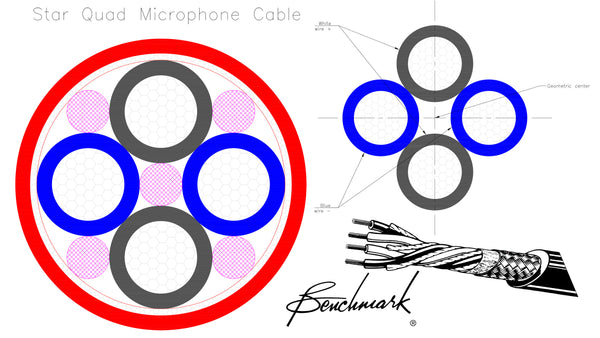
If four-conductor star-quad cable is used, the rejection of magnetic interference can be improved by about 20 to 50 dB compared to standard 2-conductor balanced cable. Star-quad cable uses two conductors for the + audio and two for the – audio. The precise geometric configuration of these conductors causes an equal common-mode pick-up of magnetic interference on both of the + and – conductor pairs. This magnetically-induced common-mode voltage will be rejected if the balanced receiver has a good CMRR.
In practice, star-quad cable is rarely needed for short line-level balanced interfaces, but it is almost always beneficial on microphone feeds. Nevertheless, star-quad cable provides an extra margin against magnetic inference when it is used with line-level balanced interfaces. For this reason, Benchmark recommends star-quad cable for all balanced interconnections. Star-quad cables are good insurance against unexpected sources of magnetic interference.
THERMAL NOISE (JOHNSON NOISE)
Every electrical component produces a certain amount of thermal noise (known as Johnson noise). This includes passive components such as resistors. Yes, passive components produce electrical noise! This noise is caused by the thermally-induced random motion of electrons.
For example, a 10 k Ohm resistor produces a noise level of -112 dBu over the audio band at room temperature. If you want to achieve a 130 dB SNR through this 10 k resistor, the signal level will need to be 130 dB higher than -112 dBu which is 18 dBu. If you are using consumer-level 2 Vrms (8.24 dBu) unbalanced signals, you will be about 10 dB short of achieving a 130 dB SNR after the signal passes through a 10 k resistor. If you want to achieve a higher SNR, you have two choices; reduce the value of the resistor, or increase the signal level.
Any practical audio circuit contains many resistors. The noise contributions of each resistor are cumulative. For this reason, drive impedances must be kept low and signal levels must be kept high. 2 Vrms consumer unbalanced interfaces are woefully inadequate. Unbalanced interfaces will usually limit the SNR to about 100 dB to 110 dB in a very well engineered product. Consumer-grade products often deliver an SNR of just 80 to 100 dB over unbalanced interfaces.
THE MYTH OF «UNBALANCED» HEADPHONES
This discussion would not be complete without mentioning that there is no such thing as an unbalanced headphone transducer (with the possible exception of DC-biased electrostatic headphones such as those manufactured by Stax).
Headphone transducers respond to the voltage difference between the two wires that feed them. They have perfect rejection of common-mode interference because there is no path to ground or to any other conductor. In other words, there is no path for ground loops.
Headphone transducers are electrically isolated from everything other than the two wires that feed them. It doesn’t matter if both conductors are driven differentially or if only one conductor is driven. The headphone transducer will reject common-mode noise.
There are some advantages to using separate wires to feed the left and right transducers, and there are some advantages to using XLR connectors instead of TRS headphone jacks, but none of these have anything to do with balanced vs. unbalanced drive. Balanced drive can provide twice the audio voltage for a given power supply voltage. XLR connectors often provide better electrical connections than TRS jacks. A separate return pin for the left and right channels can reduce crosstalk but channel separation is not really a concern with headphone listening.
In the context of this paper it is important to understand that headphone transducers always behave like perfect balanced inputs. It doesn’t matter how they are driven. Headphone transducers provide perfect rejection of common-mode noise because they only have wires. The current flowing through these wires will be equal and opposite because there is no other path for the electrons to flow.
THE MYTH OF «BALANCED» AES DIGITAL INTERFACES
In the early days of digital audio, the Audio Engineering Society (AES) decided that it would be handy to use existing analog XLR cabling to carry digital audio. In my opinion, this was a really bad idea!
Balanced connections provide no advantage with digital audio signals. Digital signals provide substantial immunity to noise. The data format used to carry digital audio was designed so that it would have no spectral content at audio frequencies. This feature allows the use of a simple high-pass filter to remove AC line-frequency interference.
Digital pulses produce substantial energy at RF frequencies. The shape of these pulses is only preserved when the cable has a controlled impedance and is terminated with resistive loads that match the cable impedance. Existing analog XLR cables had a variety of impedances and these impedances were not well controlled. Analog cables proved to be completely unreliable for digital signals and special digital XLR cables had to be created. So much for using existing cables! We now have analog and digital audio cables that look nearly identical. Digital cables are acceptable for analog audio, but analog cables cannot be used for digital audio.
The AES initially gave us a standard (AES3) for digital audio using XLR connectors and special 110-Ohm cable. But, it has been shown that coaxial cables provide better signal integrity over long transmission distances. Coaxial cables support cable runs as long as 1000 m while the 110-Ohm cable is limited to about 100 m. The video industry created a separate standard for digital audio over 75-ohm coax. As a result, the AES3 standard was updated to include digital audio over coaxial cable.
Given a choice, we would strongly recommend using unbalanced coaxial digital connections instead of balanced XLR digital connections when making long cable runs (over about 50 m). Some professional products use BNC coaxial connectors instead of RCA connectors. Consumer and professional digital audio formats are designed to talk to each other. Simple adapters can be used to connect RCA and BNC connectors. Transformers are required when adapting between balanced and unbalanced digital audio connectors.
TYPICAL PERFORMANCE OF AUDIO INTERFACES
Based on what I have seen while testing audio products in the lab, I have attempted to put together some typical performance numbers for audio interfaces. These are only approximate numbers, and is is possible to do better with careful engineering. Nevertheless, I believe these are fairly typical perfomance numbers.
- Unbalanced 2 Vrms interfaces are rarely capable of delivering an SNR better than 100 dB (the SNR equivalent of a 17-bit digital system).
- Consumer-grade 4 Vrms balanced interfaces may deliver an SNR up to about 125 dB (the SNR equivalent of a 21-bit digital system).
- Professional-grade 24 dBu balanced interfaces may deliver an SNR up to about 135 dB (the SNR equivalent of a 23-bit digital system).
As a general rule, professional-grade balanced interfaces are the only interfaces that can deliver performance that matches that of today’s best converters and amplifiers. In contrast, unbalanced interfaces tend to limit a system to CD-quality performance.
SUMMARY
Professional-grade balanced analog audio interfaces can provide a 12 to 16 dB SNR advantage over unbalanced interfaces due to the high +24 dBu signal levels used on balanced interfaces. Consumer-grade balanced interfaces can only provide 3 to 6 dB SNR advantage due to the relatively low +14 dBu (4 Vrms) signal levels.
In addition, the differential amplifier or transformer in a balanced input can provide an incredible 50 to 100 dB rejection of ground-loop interference. This is usually sufficient to reduce ground-loop interference to completely inaudible levels.
In an unbalanced interface, the shared use of the shield places ground-loop currents in the audio path. Unbalanced interfaces are very sensitive to ground currents flowing between audio components. This is not a problem with balanced interfaces due to the use of dedicated audio conductors.
Copper braid and foil layers provide shielding against RF interference. In a balanced cable, the shield does not carry the audio signal. The audio conductors are fully surrounded by the shield but are electrically isolated from the shield. In an unbalanced system, the RF shield also serves as the audio ground. This dual use of the RF shield, in an unbalanced system, causes a slight increase in susceptibility to RF interference.
Copper braid and foil shields do not provide any protection against magnetic interference. Magnetic fields easily pass through copper and foil. If star-quad cables are used in a balanced system, magnetic interference can be rejected by the CMRR of the balanced input receiver. In a balanced system, 4-conductor star-quad cables can reduce magnetic interference by 20 to 50 dB when compared to standard two-conductor balanced cables.
These numbers should be hard to ignore, but the hi-fi industry has been slow to change. Many high-end audio products still are not equipped with balanced interfaces. Others have consumer-grade 4 Vrms balanced interfaces. These are a partial step in the right direction.
The facts show that it is virtually impossible to achieve state-of-the-art audio performance using unbalanced interfaces. We see this in the lab when we measure balanced and unbalanced interfaces under ideal well-controlled conditions. Outside, in the real world, the advantages of balanced interfaces are larger than a set of balanced vs. unbalanced specifications would indicate on a product data sheet. The differences can be extremely large when ground loops, RF interference, and magnetic interference are encountered in a typical audio system.
Our recommendation? Avoid unbalanced (RCA) analog interfaces whenever possible! Look for professional-grade balanced interfaces when buying audio products. Look for CMRR specifications on balanced inputs. Consider replacing audio devices that do not support balanced interconnects. These unbalanced-only devices are probably a weak link in your audio chain.
ADDITIONAL READING
 «The Importance of Star-Quad Microphone Cable» – Benchmark Application Note, John Siau
 «Evaluating Microphone Cable Performance & Specifications» (12-page test report)